The thumbnail image is created by chatGPT-4o
This content explains how to to install FeniCSx using Spack on HPC systems (ALCF Polaris) and is based on the FeniCSx tutorial (https://jsdokken.com/dolfinx-tutorial/index.html).
1. Install Spack and FeniCSx environment
“Spack is a package management tool designed to support multiple versions and configurations of software on a wide variety of platforms and environments. It was designed for large supercomputing centers, where many users and application teams share common installations of software on clusters with exotic architectures, using libraries that do not have a standard ABI. Spack is non-destructive: installing a new version does not break existing installations, so many configurations can coexist on the same system.”
(https://spack.readthedocs.io/en/latest/)
git clone https://github.com/spack/spack.git
. ./spack/share/spack/setup-env.sh
spack env create fenicsx-env
spack env activate fenicsx-env
spack add fenics-dolfinx+adios2 py-fenics-dolfinx cflags="-O3" fflags="-O3"
spack add py-torch+cuda cuda_arc=80 (or cuda_arch=80)
spack add py-pip
spack install
For NVIDIA A100 GPU, cuda_arc = 80
Information about cuda_arc : (https://arnon.dk/matching-sm-architectures-arch-and-gencode-for-various-nvidia-cards/)
When having compiler path errors, change the programming environment to PrgEnv-nvhpc or PrgEnv-nvidia using following:
module load PrgEnv-nvhpc
or
module load PrgEnv-nvidia
(the name of the Programming environment may vary depending on the HPC system)
install gmsh
spack add gmsh
spack install gmsh

pip install gmsh
install mpi4torch
pip install mpi4torch --no-build-isolation
install torch_geometric
pip install torch_geometric
pip install torch-scatter torch-sparse torch-cluster torch-spline-conv -f https://data.pyg.org/whl/torch-2.6.0+cu121.html
To use adios4dolfinx for writing/reading checkpoints, use following .yaml file:
# This is a Spack Environment file.
#
# It describes a set of packages to be installed, along with
# configuration settings.
spack:
  # add package specs to the `specs` list
  specs:
  - fenics-dolfinx+adios2
  - py-fenics-dolfinx cflags=-O3 fflags=-O3
  - py-torch+cuda cuda_arch=80
  - py-pip
  - gmsh
  - adios2+python
  view: true
  concretizer:
    unify: true
install adios4dolfinx:
pip install adios4dolfinx
When python cannot find the python bind adios2, add these following lines at the beginning of the code:
import sys
sys.path.append("/lus/grand/projects/NeuralDE/hjkim/spack/opt/spack/linux-sles15-zen3/gcc-12.3.0/adios2-2.10.2-txcx5uunmtwgkgv55bbe7ehufkl522no/venv-1.0-5aqdxfkkynjgxyyywxsedw4igkv6z3xx/lib/python3.12/site-packages")
import adios4dolfinx
1.1 Install FeniCSx environment with torch
Install Fenicx and CUDA using spack and install torch-related libraries using pip
# This is a Spack Environment file.
#
# It describes a set of packages to be installed, along with
# configuration settings.
spack:
  # add package specs to the `specs` list
  specs:
  - fenics-dolfinx+adios2
  - py-fenics-dolfinx cflags=-O3 fflags=-O3
  - python@3.11
  - py-pip
  - cuda@12.4
  - cudnn
  - nccl cuda_arch=80
  - gmsh
  - adios2+python
  view: true
  concretizer:
    unify: true
pip install torch==2.6.0+cu124 --index-url https://download.pytorch.org/whl/cu124
pip install mpi4torch
pip install torch_geometric
pip install pyg_lib torch_scatter torch_sparse torch_cluster torch_spline_conv -f https://data.pyg.org/whl/torch-2.6.0+cu124.html
pip install adios4dolfinx
When python cannot find the python bind adios2, add these following lines at the beginning of the code:
hjkim@x3003c0s7b1n0:/grand/NeuralDE/hjkim/FeniCSx/NS> spack find -p adios2
==> In environment MLFenicsx
==> 9 root specs
[+] adios2+python  [+] cuda@12.4  [+] cudnn  [+] fenics-dolfinx+adios2  [+] gmsh  [+] nccl cuda_arch=80  [+] py-fenics-dolfinx cflags=-O3 fflags=-O3   [+] py-pip  [+] python@3.11

-- linux-sles15-zen3 / gcc@12.3.0 -------------------------------
adios2@2.10.2  /lus/grand/projects/NeuralDE/hjkim/spack/opt/spack/linux-sles15-zen3/gcc-12.3.0/adios2-2.10.2-qrwswoq6eurw7umm62hlecac3ck4ic6w
import sys
sys.path.append("/lus/grand/projects/NeuralDE/hjkim/spack/opt/spack/linux-sles15-zen3/gcc-12.3.0/adios2-2.10.2-qrwswoq6eurw7umm62hlecac3ck4ic6w/venv-1.0-6tlcx5kn3anm6pl5qj5stfe3xoptbag2/lib/python3.11/site-packages")
import adios4dolfinx
2. Solve 2D Poisson equation
2.1. Code
from mpi4py import MPI
from dolfinx import mesh
import socket
import time


comm = MPI.COMM_WORLD
rank = comm.Get_rank()
size = comm.Get_size()

print(f"Hello from rank {rank} out of {size} processes")


domain = mesh.create_unit_square(MPI.COMM_WORLD, 1024, 1024, mesh.CellType.quadrilateral)

from dolfinx.fem import functionspace
V = functionspace(domain, ("Lagrange", 1))


from dolfinx import fem
uD = fem.Function(V)
uD.interpolate(lambda x: 1 + x[0]**2 + 2 * x[1]**2)


import numpy
# Create facet to cell connectivity required to determine boundary facets
tdim = domain.topology.dim
fdim = tdim - 1
domain.topology.create_connectivity(fdim, tdim)
boundary_facets = mesh.exterior_facet_indices(domain.topology)


boundary_dofs = fem.locate_dofs_topological(V, fdim, boundary_facets)
bc = fem.dirichletbc(uD, boundary_dofs)


import ufl
u = ufl.TrialFunction(V)
v = ufl.TestFunction(V)


from dolfinx import default_scalar_type
f = fem.Constant(domain, default_scalar_type(-6))


a = ufl.dot(ufl.grad(u), ufl.grad(v)) * ufl.dx
L = f * v * ufl.dx


if rank == 0:
    start = time.time()

from dolfinx.fem.petsc import LinearProblem
problem = LinearProblem(a, L, bcs=[bc], petsc_options={"ksp_type": "preonly", "pc_type": "lu"})
uh = problem.solve()

MPI.COMM_WORLD.Barrier()

if rank ==0:
    print(f'time = {time.time()-start}')

V2 = fem.functionspace(domain, ("Lagrange", 2))
uex = fem.Function(V2)
uex.interpolate(lambda x: 1 + x[0]**2 + 2 * x[1]**2)


L2_error = fem.form(ufl.inner(uh - uex, uh - uex) * ufl.dx)
error_local = fem.assemble_scalar(L2_error)
error_L2 = numpy.sqrt(domain.comm.allreduce(error_local, op=MPI.SUM))


error_max = numpy.max(numpy.abs(uD.x.array-uh.x.array))
# Only print the error on one process
if domain.comm.rank == 0:
    print(f"Error_L2 : {error_L2:.2e}")
    print(f"Error_max : {error_max:.2e}")


from dolfinx import io
from pathlib import Path
results_folder = Path("results")
results_folder.mkdir(exist_ok=True, parents=True)
filename = results_folder / "fundamentals"
with io.VTXWriter(domain.comm, filename.with_suffix(".bp"), [uh]) as vtx:
    vtx.write(0.0)
with io.XDMFFile(domain.comm, filename.with_suffix(".xdmf"), "w") as xdmf:
    xdmf.write_mesh(domain)
    xdmf.write_function(uh)
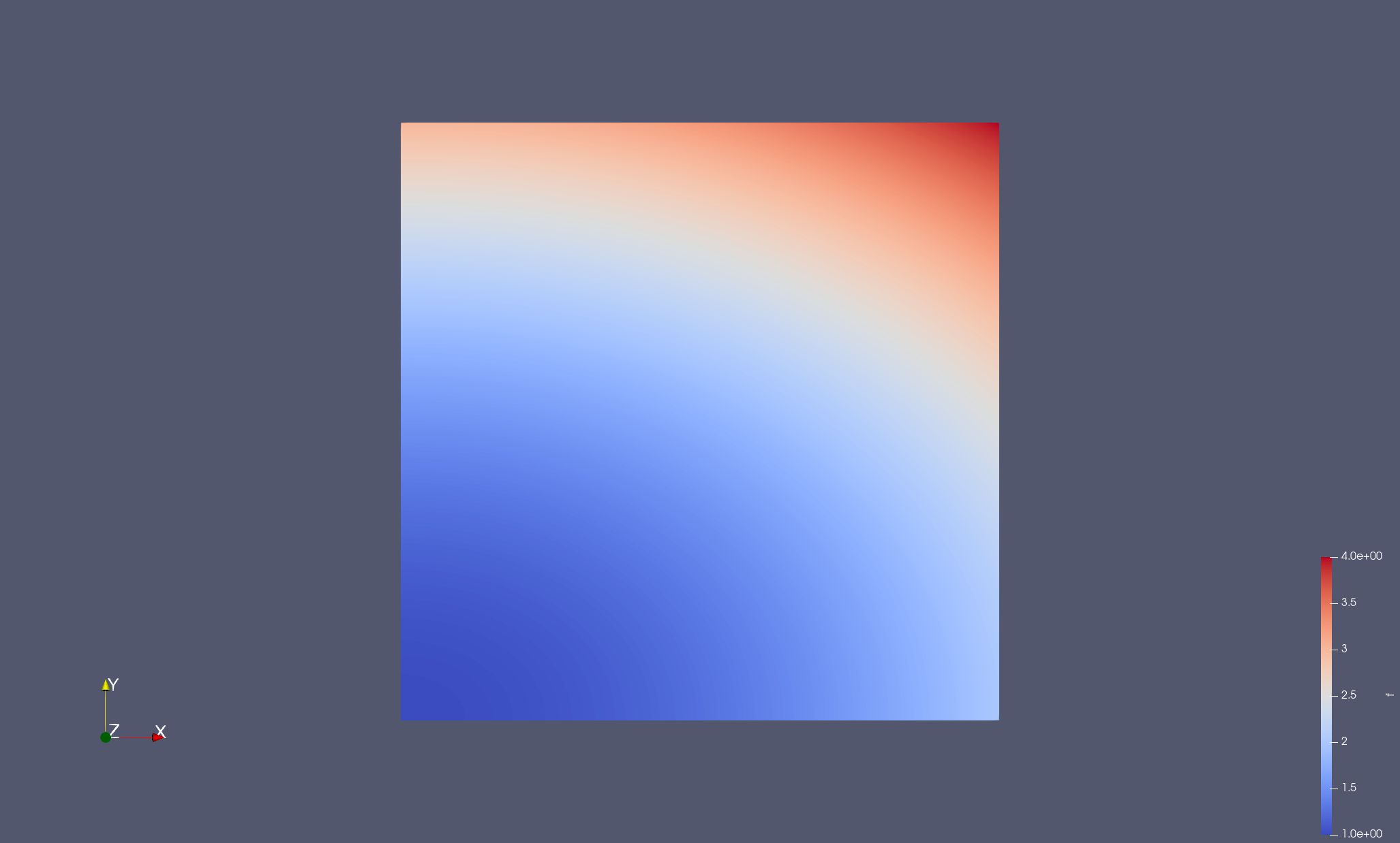
2.2. Results
mpirun --oversubscribe -n 32 python poisson.py
the number of MPI ranks: 32
computation time = 9.24938178062439 sec
Error_L2 : 5.03e-07
Error_max : 6.44e-11
python poisson.py
the number of MPI ranks: 1
computation time = 21.489859342575073 sec
Error_L2 : 5.03e-07
Error_max : 6.11e-11
3. Incompressible Navier-Stokes equation: flow around cylinder
3.1. Code
import gmsh
import os
import numpy as np
import matplotlib.pyplot as plt
import tqdm.autonotebook

from mpi4py import MPI
from petsc4py import PETSc

from basix.ufl import element

from dolfinx.cpp.mesh import to_type, cell_entity_type
from dolfinx.fem import (Constant, Function, functionspace,
                         assemble_scalar, dirichletbc, form, locate_dofs_topological, set_bc)
from dolfinx.fem.petsc import (apply_lifting, assemble_matrix, assemble_vector,
                               create_vector, create_matrix, set_bc)
from dolfinx.graph import adjacencylist
from dolfinx.geometry import bb_tree, compute_collisions_points, compute_colliding_cells
from dolfinx.io import (VTXWriter, distribute_entity_data, gmshio)
from dolfinx.mesh import create_mesh, meshtags_from_entities
from ufl import (FacetNormal, Identity, Measure, TestFunction, TrialFunction,
                 as_vector, div, dot, ds, dx, inner, lhs, grad, nabla_grad, rhs, sym, system)

gmsh.initialize()

L = 2.2
H = 0.41
c_x = c_y = 0.2
r = 0.05
gdim = 2
mesh_comm = MPI.COMM_WORLD
model_rank = 0
if mesh_comm.rank == model_rank:
    rectangle = gmsh.model.occ.addRectangle(0, 0, 0, L, H, tag=1)
    obstacle = gmsh.model.occ.addDisk(c_x, c_y, 0, r, r)


if mesh_comm.rank == model_rank:
    fluid = gmsh.model.occ.cut([(gdim, rectangle)], [(gdim, obstacle)])
    gmsh.model.occ.synchronize()


fluid_marker = 1
if mesh_comm.rank == model_rank:
    volumes = gmsh.model.getEntities(dim=gdim)
    assert (len(volumes) == 1)
    gmsh.model.addPhysicalGroup(volumes[0][0], [volumes[0][1]], fluid_marker)
    gmsh.model.setPhysicalName(volumes[0][0], fluid_marker, "Fluid")


inlet_marker, outlet_marker, wall_marker, obstacle_marker = 2, 3, 4, 5
inflow, outflow, walls, obstacle = [], [], [], []
if mesh_comm.rank == model_rank:
    boundaries = gmsh.model.getBoundary(volumes, oriented=False)
    for boundary in boundaries:
        center_of_mass = gmsh.model.occ.getCenterOfMass(boundary[0], boundary[1])
        if np.allclose(center_of_mass, [0, H / 2, 0]):
            inflow.append(boundary[1])
        elif np.allclose(center_of_mass, [L, H / 2, 0]):
            outflow.append(boundary[1])
        elif np.allclose(center_of_mass, [L / 2, H, 0]) or np.allclose(center_of_mass, [L / 2, 0, 0]):
            walls.append(boundary[1])
        else:
            obstacle.append(boundary[1])
    gmsh.model.addPhysicalGroup(1, walls, wall_marker)
    gmsh.model.setPhysicalName(1, wall_marker, "Walls")
    gmsh.model.addPhysicalGroup(1, inflow, inlet_marker)
    gmsh.model.setPhysicalName(1, inlet_marker, "Inlet")
    gmsh.model.addPhysicalGroup(1, outflow, outlet_marker)
    gmsh.model.setPhysicalName(1, outlet_marker, "Outlet")
    gmsh.model.addPhysicalGroup(1, obstacle, obstacle_marker)
    gmsh.model.setPhysicalName(1, obstacle_marker, "Obstacle")


# Create distance field from obstacle.
# Add threshold of mesh sizes based on the distance field
# LcMax -                  /--------
#                      /
# LcMin -o---------/
#        |         |       |
#       Point    DistMin DistMax
res_min = r / 3
if mesh_comm.rank == model_rank:
    distance_field = gmsh.model.mesh.field.add("Distance")
    gmsh.model.mesh.field.setNumbers(distance_field, "EdgesList", obstacle)
    threshold_field = gmsh.model.mesh.field.add("Threshold")
    gmsh.model.mesh.field.setNumber(threshold_field, "IField", distance_field)
    gmsh.model.mesh.field.setNumber(threshold_field, "LcMin", res_min)
    gmsh.model.mesh.field.setNumber(threshold_field, "LcMax", 0.25 * H)
    gmsh.model.mesh.field.setNumber(threshold_field, "DistMin", r)
    gmsh.model.mesh.field.setNumber(threshold_field, "DistMax", 2 * H)
    min_field = gmsh.model.mesh.field.add("Min")
    gmsh.model.mesh.field.setNumbers(min_field, "FieldsList", [threshold_field])
    gmsh.model.mesh.field.setAsBackgroundMesh(min_field)


if mesh_comm.rank == model_rank:
    gmsh.option.setNumber("Mesh.Algorithm", 8)
    gmsh.option.setNumber("Mesh.RecombinationAlgorithm", 2)
    gmsh.option.setNumber("Mesh.RecombineAll", 1)
    gmsh.option.setNumber("Mesh.SubdivisionAlgorithm", 1)
    gmsh.model.mesh.generate(gdim)
    gmsh.model.mesh.setOrder(2)
    gmsh.model.mesh.optimize("Netgen")


mesh, _, ft = gmshio.model_to_mesh(gmsh.model, mesh_comm, model_rank, gdim=gdim)
ft.name = "Facet markers"


t = 0
T = 8                       # Final time
dt = 1 / 1600                 # Time step size
num_steps = int(T / dt)
k = Constant(mesh, PETSc.ScalarType(dt))
mu = Constant(mesh, PETSc.ScalarType(0.001))  # Dynamic viscosity
rho = Constant(mesh, PETSc.ScalarType(1))     # Density
dolfinx.fem.Constant(domain, c: ndarray | Sequence | floating | complexfloating)
Bases: Constant
A constant with respect to a domain.
Parameters:
domain– DOLFINx or UFL meshc– Value of the constant.
v_cg2 = element("Lagrange", mesh.topology.cell_name(), 2, shape=(mesh.geometry.dim, ))
s_cg1 = element("Lagrange", mesh.topology.cell_name(), 1)
V = functionspace(mesh, v_cg2)
Q = functionspace(mesh, s_cg1)

fdim = mesh.topology.dim - 1
basix.ufl.element(family: ElementFamily | str, cell: CellType | str, degree: int, lagrange_variant: LagrangeVariant = LagrangeVariant.unset, dpc_variant: DPCVariant = DPCVariant.unset, discontinuous: bool = False, shape: tuple[int, ...] | None = None, symmetry: bool | None = None, dof_ordering: list[int] | None = None, dtype: dtype[Any] | None | type[Any] | _SupportsDType[dtype[Any]] | str | tuple[Any, int] | tuple[Any, SupportsIndex | Sequence[SupportsIndex]] | list[Any] | _DTypeDict | tuple[Any, Any] = None) → _ElementBase
Create a UFL compatible element using Basix.
Parameters:
family– Element family/type.cell– Element cell type.degree– Degree of the finite element.lagrange_variant– Variant of Lagrange to be used.dpc_variant– Variant of DPC to be used.discontinuous– If True, the discontinuous version of the element is created.shape– Value shape of the element. For scalar-valued families, this can be used to create vector and tensor elements.symmetry– Set to True if the tensor is symmetric. Valid for rank 2 elements only.dof_ordering– Ordering of dofs for ElementDofLayout.dtype– Floating point data type.
Returns:
UFL finite element.
# Define boundary conditions


class InletVelocity():
    def __init__(self, t):
        self.t = t

    def __call__(self, x):
        values = np.zeros((gdim, x.shape[1]), dtype=PETSc.ScalarType)
        values[0] = 4 * 1.5 * np.sin(self.t * np.pi / 8) * x[1] * (0.41 - x[1]) / (0.41**2)
        return values


# Inlet
u_inlet = Function(V)
inlet_velocity = InletVelocity(t)
u_inlet.interpolate(inlet_velocity)
bcu_inflow = dirichletbc(u_inlet, locate_dofs_topological(V, fdim, ft.find(inlet_marker)))
# Walls
u_nonslip = np.array((0,) * mesh.geometry.dim, dtype=PETSc.ScalarType)
bcu_walls = dirichletbc(u_nonslip, locate_dofs_topological(V, fdim, ft.find(wall_marker)), V)
# Obstacle
bcu_obstacle = dirichletbc(u_nonslip, locate_dofs_topological(V, fdim, ft.find(obstacle_marker)), V)
bcu = [bcu_inflow, bcu_obstacle, bcu_walls]
# Outlet
bcp_outlet = dirichletbc(PETSc.ScalarType(0), locate_dofs_topological(Q, fdim, ft.find(outlet_marker)), Q)
bcp = [bcp_outlet]
dolfinx.fem.DirichletBC(bc)
Bases: object
Representation of Dirichlet boundary condition which is imposed on a linear system.
Note:
Dirichlet boundary conditions should normally be constructed usingfem.dirichletbc()
and not using this class initializer. This class is combined with different base classes
that depend on the scalar type of the boundary condition.
Parameters
value– Lifted boundary values function. It can be Function, array or constant valuesdofs– Local indices of degrees of freedom in the function space to which the boundary condition applies.- Expects an array of size
(number of dofs, 2)if function space of the problem,V, is passed. - Otherwise, assumes function space of the problem is the same as the function space of the boundary values function.
- Expects an array of size
V– Function space of a problem to which boundary conditions are applied.
Returns:
A representation of the boundary condition for modifying linear systems.
u = TrialFunction(V)
v = TestFunction(V)
u_ = Function(V)
u_.name = "u"
u_s = Function(V)
u_n = Function(V)
u_n1 = Function(V)
p = TrialFunction(Q)
q = TestFunction(Q)
p_ = Function(Q)
p_.name = "p"
phi = Function(Q)


f = Constant(mesh, PETSc.ScalarType((0, 0)))
F1 = rho / k * dot(u - u_n, v) * dx
F1 += inner(dot(1.5 * u_n - 0.5 * u_n1, 0.5 * nabla_grad(u + u_n)), v) * dx
F1 += 0.5 * mu * inner(grad(u + u_n), grad(v)) * dx - dot(p_, div(v)) * dx
F1 += dot(f, v) * dx
a1 = form(lhs(F1))
L1 = form(rhs(F1))
A1 = create_matrix(a1)
b1 = create_vector(L1)

a2 = form(dot(grad(p), grad(q)) * dx)
L2 = form(-rho / k * dot(div(u_s), q) * dx)
A2 = assemble_matrix(a2, bcs=bcp)
A2.assemble()
b2 = create_vector(L2)


a3 = form(rho * dot(u, v) * dx)
L3 = form(rho * dot(u_s, v) * dx - k * dot(nabla_grad(phi), v) * dx)
A3 = assemble_matrix(a3)
A3.assemble()
b3 = create_vector(L3)
ufl.inner(a, b)[source]
Take the inner product of a and b.
The complex conjugate of the second argument is taken.
ufl.lhs(form)
Get the left hand side.
Given a combined bilinear and linear form, extract the left hand side (bilinear form part).
Example: a = uvdx + fvdx a = lhs(a) -> uvdx
dolfinx.fem.form(form: typing.Union[ufl.Form, typing.Iterable[ufl.Form]], dtype: npt.DTypeLike = <class 'numpy.float64'>, form_compiler_options: typing.Optional[dict] = None, jit_options: typing.Optional[dict] = None, entity_maps: typing.Optional[dict[Mesh, np.typing.NDArray[np.int32]]] = None)[source]
Create a Form or an array of Forms.
Parameters
form– A UFL form or list(s) of UFL forms.dtype– Scalar type to use for the compiled form.form_compiler_options– See ffcx_jitjit_options– See ffcx_jit.entity_maps– If any trial functions, test functions, or coefficients in the form are not defined over the same mesh as the integration domain, entity_maps must be supplied. For each key (a mesh, different to the integration domain mesh) a map should be provided relating the entities in the integration domain mesh to the entities in the key mesh e.g. for a key-value pair (msh, emap) in entity_maps, emap[i] is the entity in msh corresponding to entity i in the integration domain mesh.
Returns:
Compiled finite element Form.
dolfinx.fem.petsc.create_matrix(a: Form, mat_type=None)→ Mat[source]
Create a PETSc matrix that is compatible with a bilinear form.
Note:
Due to subtle issues in the interaction between petsc4py memory management and the Python garbage collector, it is recommended that the method PETSc.Mat.destroy() is called on the returned object once the object is no longer required. Note that PETSc.Mat.destroy() is collective over the object’s MPI communicator.
Parameters
a– A bilinear form.mat_type– The PETSc matrix type (MatType).
Returns:
A PETSc matrix with a layout that is compatible with a.
dolfinx.fem.petsc.create_vector(L: Form)→ Vec[source]
Create a PETSc vector that is compatible with a linear form.
Parameters
L– A linear form.
Returns:
A PETSc vector with a layout that is compatible with L.
dolfinx.fem.petsc.assemble_matrix(A: Mat, a: Form, bcs: list[DirichletBC] = [], diagonal: float = 1.0, constants=None, coeffs=None)→ Mat
Assemble bilinear form into a matrix.
The returned matrix is not finalised, i.e. ghost values are not accumulated.
Note:
The returned matrix is not ‘assembled’, i.e. ghost contributions have not been communicated. Should be followd by $assemble()$.
Parameters
a– Bilinear form to assembled into a matrix.bc– Dirichlet boundary conditions applied to the system.diagonal– Value to set on the matrix diagonal for Dirichlet boundary condition constrained degrees-of-freedom belonging to the same trial and test space.constants– Constants appearing the in the form.coeffs– Coefficients appearing the in the form.
Returns:
Matrix representing the bilinear form.
# Solver for step 1
solver1 = PETSc.KSP().create(mesh.comm)
solver1.setOperators(A1)
solver1.setType(PETSc.KSP.Type.BCGS)
pc1 = solver1.getPC()
pc1.setType(PETSc.PC.Type.JACOBI)

# Solver for step 2
solver2 = PETSc.KSP().create(mesh.comm)
solver2.setOperators(A2)
solver2.setType(PETSc.KSP.Type.MINRES)
pc2 = solver2.getPC()
pc2.setType(PETSc.PC.Type.HYPRE)
pc2.setHYPREType("boomeramg")

# Solver for step 3
solver3 = PETSc.KSP().create(mesh.comm)
solver3.setOperators(A3)
solver3.setType(PETSc.KSP.Type.CG)
pc3 = solver3.getPC()
pc3.setType(PETSc.PC.Type.SOR)
Krylov Subspace Solver (KSP) & Preconditioner setting
PETSc.KSP().create(mesh.comm)solver.setOperators(A)-
solver.setType(PETSc.KSP.Type.BCGS) solver.getPC()solver.getPC().setType(PETSc.PC.Type.
petsc4py.PETSc.KSP
Class: petsc4py.PETSc.KSP
Bases: Object
Overview
KSP is an abstract PETSc object that manages all Krylov methods.
This object handles the linear solves in PETSc, including direct solvers that do not use Krylov accelerators.
Notes
When a direct solver is used without a Krylov solver, the
KSPobject is still utilized.
In this case,Type.PREONLYis set, meaning only the application of the preconditioner is used as the linear solver.
create(comm=None)
Create the KSP context.
Collective.
Paramters:
comm(Comm|None)
Returns:
Self
setOperators(A=None, P=None)
Set matrix associated with the linear system.
Collective.
Set the matrix associated with the linear system and a (possibly) different one from which the preconditioner will be built.
Paramters:
A(Mat|None): Matrix that defines the linear system.P(Mat|None): Matrix to be used in constructing the preconditioner, usually the same as A
Returns:
None
setType(ksp_type)
Build the KSP data structure for a particular Type.
Logically collective.
Paramters:
ksp_type (Type | str): KSP Type object
Returns:
None
getPC()
Return the preconditioner.
Not collective.
Returns:
PC
petsc4py.PETSc.PC
Class: petsc4py.PETSc.PC
Bases: Object
Overview
Preconditioners.
PC is described in the PETSc manual. Calling the PC with a vector as an argument will apply the preconditioner as shown in the example below.
setType(pc_type)
Set the preconditioner type.
Collective.
Paramters:
pc_type (Type | str): The preconditioner type.
Returns:
None
setType(pc_type)
Set the preconditioner type.
Collective.
Paramters:
pc_type (Type | str): The preconditioner type.
Returns:
None
setHYPREType(hypretype)
Set the Type.HYPRE type.
Collective.
Paramters:
hypretype (str): The name of the type, one of"euclid","pilut","parasails","boomeramg","ams","ads"
Returns:
None
n = -FacetNormal(mesh)  # Normal pointing out of obstacle
dObs = Measure("ds", domain=mesh, subdomain_data=ft, subdomain_id=obstacle_marker)
u_t = inner(as_vector((n[1], -n[0])), u_)
drag = form(2 / 0.1 * (mu / rho * inner(grad(u_t), n) * n[1] - p_ * n[0]) * dObs)
lift = form(-2 / 0.1 * (mu / rho * inner(grad(u_t), n) * n[0] + p_ * n[1]) * dObs)
if mesh.comm.rank == 0:
    C_D = np.zeros(num_steps, dtype=PETSc.ScalarType)
    C_L = np.zeros(num_steps, dtype=PETSc.ScalarType)
    t_u = np.zeros(num_steps, dtype=np.float64)
    t_p = np.zeros(num_steps, dtype=np.float64)
ufl.classes.FacetNormal(domain)
The outwards pointing normal vector of the current facet.
ufl.Measure(integral_type, domain=None, subdomain_id='everywhere', metadata=None, subdomain_data=None)[source]
Representation of an integration measure.
The Measure object holds information about integration properties to be transferred to a Form on multiplication with a scalar expression.
tree = bb_tree(mesh, mesh.geometry.dim)
points = np.array([[0.15, 0.2, 0], [0.25, 0.2, 0]])
cell_candidates = compute_collisions_points(tree, points)
colliding_cells = compute_colliding_cells(mesh, cell_candidates, points)
front_cells = colliding_cells.links(0)
back_cells = colliding_cells.links(1)
if mesh.comm.rank == 0:
    p_diff = np.zeros(num_steps, dtype=PETSc.ScalarType)
dolfinx.geometry.bb_tree(mesh: Mesh, dim: int, entities: Optional[npt.NDArray[np.int32]] = None, padding: float = 0.0)→ BoundingBoxTree[source]
Create a bounding box tree for use in collision detection.
Paramters:
mesh: The mesh.dim: Dimension of the mesh entities to build bounding box for.entities: List of entity indices (local to process). If not supplied, all owned and ghosted entities are used.padding: Padding for each bounding box.
Returns:
Bounding box tree.
dolfinx.geometry.compute_collisions_points(tree: BoundingBoxTree, x: ndarray[Any, dtype[floating]])→ AdjacencyList_int32
Compute collisions between points and leaf bounding boxes.
Bounding boxes can overlap, therefore points can collide with more than one box.
Paramters:
tree: Bounding box treex: Points
Returns:
For each point, the bounding box leaves that collide with the point.
dolfinx.geometry.compute_colliding_cells(mesh: Mesh, candidates: AdjacencyList_int32, x: npt.NDArray[np.floating])
From a mesh, find which cells collide with a set of points.
Paramters:
mesh: The meshcandidate_cells: Adjacency list of candidate colliding cells for the ith point inx.points: The points to check for collision
Returns:
Adjacency list where the ith node is the list of entities that collide with the ith point.
links
Links (edges) of a node
from pathlib import Path
folder = Path("results")
folder.mkdir(exist_ok=True, parents=True)
vtx_u = VTXWriter(mesh.comm, "dfg2D-3-u.bp", [u_], engine="BP4")
vtx_p = VTXWriter(mesh.comm, "dfg2D-3-p.bp", [p_], engine="BP4")
vtx_u.write(t)
vtx_p.write(t)
progress = tqdm.autonotebook.tqdm(desc="Solving PDE", total=num_steps)
for i in range(num_steps):
    progress.update(1)
    # Update current time step
    t += dt
    # Update inlet velocity
    inlet_velocity.t = t
    u_inlet.interpolate(inlet_velocity)

    # Step 1: Tentative velocity step
    A1.zeroEntries()
    assemble_matrix(A1, a1, bcs=bcu)
    A1.assemble()
    with b1.localForm() as loc:
        loc.set(0)
    assemble_vector(b1, L1)
    apply_lifting(b1, [a1], [bcu])
    b1.ghostUpdate(addv=PETSc.InsertMode.ADD_VALUES, mode=PETSc.ScatterMode.REVERSE)
    set_bc(b1, bcu)
    solver1.solve(b1, u_s.x.petsc_vec)
    u_s.x.scatter_forward()


    # Step 2: Pressure corrrection step
    with b2.localForm() as loc:
        loc.set(0)
    assemble_vector(b2, L2)
    apply_lifting(b2, [a2], [bcp])
    b2.ghostUpdate(addv=PETSc.InsertMode.ADD_VALUES, mode=PETSc.ScatterMode.REVERSE)
    set_bc(b2, bcp)
    solver2.solve(b2, phi.x.petsc_vec)
    phi.x.scatter_forward()

    p_.x.petsc_vec.axpy(1, phi.x.petsc_vec)
    p_.x.scatter_forward()

    # Step 3: Velocity correction step
    with b3.localForm() as loc:
        loc.set(0)
    assemble_vector(b3, L3)
    b3.ghostUpdate(addv=PETSc.InsertMode.ADD_VALUES, mode=PETSc.ScatterMode.REVERSE)
    solver3.solve(b3, u_.x.petsc_vec)
    u_.x.scatter_forward()

    # Write solutions to file
    vtx_u.write(t)
    vtx_p.write(t)

    # Update variable with solution form this time step
    with u_.x.petsc_vec.localForm() as loc_, u_n.x.petsc_vec.localForm() as loc_n, u_n1.x.petsc_vec.localForm() as loc_n1:
        loc_n.copy(loc_n1)
        loc_.copy(loc_n)

    # Compute physical quantities
    # For this to work in paralell, we gather contributions from all processors
    # to processor zero and sum the contributions.
    drag_coeff = mesh.comm.gather(assemble_scalar(drag), root=0)
    lift_coeff = mesh.comm.gather(assemble_scalar(lift), root=0)
    p_front = None
    if len(front_cells) > 0:
        p_front = p_.eval(points[0], front_cells[:1])
    p_front = mesh.comm.gather(p_front, root=0)
    p_back = None
    if len(back_cells) > 0:
        p_back = p_.eval(points[1], back_cells[:1])
    p_back = mesh.comm.gather(p_back, root=0)
    if mesh.comm.rank == 0:
        t_u[i] = t
        t_p[i] = t - dt / 2
        C_D[i] = sum(drag_coeff)
        C_L[i] = sum(lift_coeff)
        # Choose first pressure that is found from the different processors
        for pressure in p_front:
            if pressure is not None:
                p_diff[i] = pressure[0]
                break
        for pressure in p_back:
            if pressure is not None:
                p_diff[i] -= pressure[0]
                break
progress.close()
vtx_u.close()
vtx_p.close()
petsc4py.PETSc.localForm()
Return a context manager for viewing ghost vectors in local form.
Logically collective.
Returns:
Context manager yielding the vector in local (ghosted) form.
dolfinx.fem.petsc.apply_lifting(b: Vec, a: list[Form], bcs: list[list[DirichletBC]], x0: list[Vec] = [], alpha: float = 1, constants=None, coeffs=None)→ None[source]
Apply the function dolfinx.fem.apply_lifting() to a PETSc Vector.
dolfinx.fem.apply_lifting(b: ndarray, a: list[Form], bcs: list[list[DirichletBC]], x0: list[ndarray] | None = None, alpha: float = 1, constants=None, coeffs=None)→ None[source]
Modify RHS vector b for lifting of Dirichlet boundary conditions.
It modifies b such that:
$b \gets b - \text{scale} \cdot A_j (g_j - x0_j)$
where j is a block (nest) index. For a non-blocked problem j = 0. The boundary conditions bcs are on the trial spaces V_j. The forms in [a] must have the same test space as L (from which b was built), but the trial space may differ. If x0 is not supplied, then it is treated as zero.
ghostUpdate(addv=None, mode=None)
Update ghosted vector entries.
Neighborwise collective.
Parameters
addv(InsertModeSpec) – Insertion mode.mode(ScatterModeSpec) – Scatter mode.
Return type:
None
dolfinx.fem.petsc.set_bc(b: Vec, bcs: list[DirichletBC], x0: Vec | None = None, alpha: float = 1)→ None[source]
Apply the function dolfinx.fem.set_bc() to a PETSc Vector.
dolfinx.fem.set_bc(b: ndarray, bcs: list[DirichletBC], x0: ndarray | None = None, scale: float = 1)→ None[source]
Insert boundary condition values into vector.
petsc4py.PETSc.KSP.solve(b, x)
Solve the linear system.
Collective.
Parameters
b (Vec)– Right hand side vector.x (Vec)– Solution vector.
Return type:
None
Note
If one uses setDM then x or b need not be passed. Use getSolution to access the solution in this case.
The operator is specified with setOperators.
solve will normally return without generating an error regardless of whether the linear system was solved or if constructing the preconditioner failed. Call getConvergedReason to determine if the solver converged or failed and why. The option -ksp_error_if_not_converged or function setErrorIfNotConverged will cause solve to error as soon as an error occurs in the linear solver. In inner solves, DIVERGED_MAX_IT is not treated as an error because when using nested solvers it may be fine that inner solvers in the preconditioner do not converge during the solution process.
The number of iterations can be obtained from its.
If you provide a matrix that has a Mat.setNullSpace and Mat.setTransposeNullSpace this will use that information to solve singular systems in the least squares sense with a norm minimizing solution.
Ax = b where b = bₚ + bₜ where bₜ is not in the range of A (and hence by the fundamental theorem of linear algebra is in the nullspace(Aᵀ), see Mat.setNullSpace.
KSP first removes bₜ producing the linear system Ax = bₚ (which has multiple solutions) and solves this to find the ∥x∥ minimizing solution (and hence it finds the solution x orthogonal to the nullspace(A). The algorithm is simply in each iteration of the Krylov method we remove the nullspace(A) from the search direction thus the solution which is a linear combination of the search directions has no component in the nullspace(A).
We recommend always using Type.GMRES for such singular systems. If nullspace(A) = nullspace(Aᵀ) (note symmetric matrices always satisfy this property) then both left and right preconditioning will work If nullspace(A) != nullspace(Aᵀ) then left preconditioning will work but right preconditioning may not work (or it may).
If using a direct method (e.g., via the KSP solver Type.PREONLY and a preconditioner such as PC.Type.LU or PC.Type.ILU, then its=1. See setTolerances for more details.
Understanding Convergence
The routines setMonitor and computeEigenvalues provide information on additional options to monitor convergence and print eigenvalue information.
dolfinx.la.Vector.scatter_forward()→ None
Update ghost entries.
petsc4py.PETSc.Vec.axpy(alpha, x)
Compute and store y = ɑ·x + y.
Logically collective.
Parameters
alpha (Scalar)– Scale factor.x (Vec)– Input vector.
Return type:
None
dolfinx.fem.assemble_scalar(M: Form, constants=None, coeffs=None)[source]
Assemble functional. The returned value is local and not accumulated across processes.
Parameters
M– The functional to compute.constants– Constants that appear in the form. If not provided, any required constants will be computed.coeffs– Coefficients that appear in the form. If not provided, any required coefficients will be computed.
Returns:
The computed scalar on the calling rank. Note
Note Passing constants and coefficients is a performance optimisation for when a form is assembled multiple times and when (some) constants and coefficients are unchanged.
To compute the functional value on the whole domain, the output of this function is typically summed across all MPI ranks.
dolfinx.fem.eval(x: Buffer | _SupportsArray[dtype[Any]] | _NestedSequence[_SupportsArray[dtype[Any]]] | bool | int | float | complex | str | bytes | _NestedSequence[bool | int | float | complex | str | bytes], cells: Buffer | _SupportsArray[dtype[Any]] | _NestedSequence[_SupportsArray[dtype[Any]]] | bool | int | float | complex | str | bytes | _NestedSequence[bool | int | float | complex | str | bytes], u=None)→ ndarray[source]
Evaluate Function at points x.
Points where x has shape (num_points, 3), and cells has shape (num_points,) and cell[i] is the index of the cell containing point x[i]. If the cell index is negative the point is ignored.
if mesh.comm.rank == 0:
    if not os.path.exists("figures"):
        os.mkdir("figures")
    num_velocity_dofs = V.dofmap.index_map_bs * V.dofmap.index_map.size_global
    num_pressure_dofs = Q.dofmap.index_map_bs * V.dofmap.index_map.size_global

    turek = np.loadtxt("bdforces_lv4")
    turek_p = np.loadtxt("pointvalues_lv4")
    fig = plt.figure(figsize=(25, 8))
    l1 = plt.plot(t_u, C_D, label=r"FEniCSx  ({0:d} dofs)".format(num_velocity_dofs + num_pressure_dofs), linewidth=2)
    l2 = plt.plot(turek[1:, 1], turek[1:, 3], marker="x", markevery=50,
                  linestyle="", markersize=4, label="FEATFLOW (42016 dofs)")
    plt.title("Drag coefficient")
    plt.grid()
    plt.legend()
    plt.savefig("figures/drag_comparison.png")

    fig = plt.figure(figsize=(25, 8))
    l1 = plt.plot(t_u, C_L, label=r"FEniCSx  ({0:d} dofs)".format(
        num_velocity_dofs + num_pressure_dofs), linewidth=2)
    l2 = plt.plot(turek[1:, 1], turek[1:, 4], marker="x", markevery=50,
                  linestyle="", markersize=4, label="FEATFLOW (42016 dofs)")
    plt.title("Lift coefficient")
    plt.grid()
    plt.legend()
    plt.savefig("figures/lift_comparison.png")

    fig = plt.figure(figsize=(25, 8))
    l1 = plt.plot(t_p, p_diff, label=r"FEniCSx ({0:d} dofs)".format(num_velocity_dofs + num_pressure_dofs), linewidth=2)
    l2 = plt.plot(turek[1:, 1], turek_p[1:, 6] - turek_p[1:, -1], marker="x", markevery=50,
                  linestyle="", markersize=4, label="FEATFLOW (42016 dofs)")
    plt.title("Pressure difference")
    plt.grid()
    plt.legend()
    plt.savefig("figures/pressure_comparison.png")
3.1. Results
python NS_2Dcylinder.py
Solving PDE: 100%|██████████████████████████████████████████████████████████████████████████████████████████████████████████████████████████████████████████████████████████████████████| 12800/12800 [09:06<00:00, 23.41it/s]
mpirun --oversubscribe -n 20 python NS_2Dcylinder.py
Solving PDE: 100%|██████████| 12800/12800 [01:30<00:00, 141.82it/s]