This content is based on “Differentiable Turbulence II” by Varun Shankar et al. ¹.

1. Adjoint method
   • Purpose
   • Derivation
     
2. Differentiable PDE solver
   • Purpose
   • Implementation

1. Adjoint method

1.1. Purpose

  The method of Lagrangian multiplier provides a way to find optimal solutions in the optimization problem with constraints. However, for complex systems like systems of PDE, it is really difficult to get the optimal solution directly from the method of Lagrangian multiplier. The Adjoint method helps to find solutions to complex optimization problems by providing a gradient of the objective function with respect to optimization variables.

1.2. Derivation

  Let’s say we have the objective function $f(x, m)$ and constraint $g(x, m)$, where x is the state variable, and m is the optimization variable. Our goal is to calculate the total derivative of the objective function with respect to the optimization variable, $\frac{df}{dm}$.

And define Lagrangian $L(x, m, \lambda)$ as follows.

\(L(x, m, \lambda) = f(x, m) + \lambda^Tg(x, m)\)
,where $\lambda$ is the adjoint variable or Lagrangian multiplier.

Sicne $g(x,m) = 0$ everywhere, $f(x,m)$ is equivalent to $L(x, m, \lambda)$, and we can choose $\lambda$ freely. Also, we can think $f(x,m)$ as $f(x(m))$.

Then, $\frac{df}{dm}$ becomes

\(\frac{df}{dm} = \frac{dL}{dm} = \frac{\partial f}{\partial x}\frac{dx}{dm} + \frac{d\lambda^T}{dm}g + \lambda^T(\frac{\partial g}{\partial m} + \frac{\partial g}{\partial x}\frac{dx}{dm})\)

Since $g(x,m)=0$, it becomes

\(\frac{df}{dm} = (\frac{\partial f}{\partial x}+\lambda^T\frac{\partial g}{\partial x})\frac{dx}{dm}+\lambda^T\frac{\partial g}{\partial m}\)

Generally, it is difficult to know $\frac{dx}{dm}$. Therefore, by setting

\(\frac{\partial f}{\partial x} + \lambda^T \frac{\partial g}{\partial x} = 0\)

we don’t need to compute $\frac{dx}{dm}$.

Then, \(\frac{df}{dm} = \lambda^T\frac{\partial g}{\partial m}\)

,which can be calculated using $\lambda$ from the above equation.

In summary, by utilizing Lagrangian and setting the adjoint variable properly, we can compute a gradient of the objective function with regard to parameters.

2. Differentiable PDE solver

2.1. Purpose

  Turbulence modeling with machine learning techniques usually has taken a-priori learning. While a-priori approach in modeling turbulence is easy to implement, it can’t guarantee accurate prediction for unseen data. This is because when a learned model is embedded into the PDE solver, numerical artifacts, such as numerical errors and temporal errors, are produced by the PDE solver. These artifacts are not included in the training process, thus deteriorating prediction capability for unseen data.

  However, differentiable PDE solver enables end-to-end training of machine learning models with backpropagation, enhancing a-posteriori prediction capability. A differentiable PDE solver can be realized by implementing a governing equation in an automatic differentiation (AD) framework, which is a necessary tool for training deep neural networks.

2.2. Implementation with the adjoint method

  The AD framework’s basic principle is that gradients of a composition of differentiable functions can be exactly computed using the chain rule. Deep neural networks are composed of straightforward operations, such as linear or pointwise nonlinear operations. Therefore, gradients can be easily computed in the training of deep neural networks using the AD framework. However, writing a PDE solver in an AD-enabled way can add enormous complexity, which makes it impractical. Instead, by implementing a vector-jacobian product using the discrete adjoint method, we can integrate a PDE solver within the AD framework.

  The basic chain rule is as follows.
$x_1=f_0(x_0)$
$x_2=f_0(x_1)$
.
.
.
$y=f_n(x_n)$

$\frac{dy}{dx_i}=\frac{dy}{dx_{i+1}}\frac{dx_{i+1}}{dx_i}=\frac{dy}{dx_{i+1}}\frac{df_i(x_i)}{dx_i}$.

 The iterative nature of the chain rule allows gradients of $y$ to be propagated backward starting from $\frac{dy}{dx_n}$. To enable backpropagation, the reverse function should be implemented in each forward operation. This reverse function is called a vector-jacobian product (VJP):

$\frac{dy}{dx_i}={f_i}^{\prime}(\frac{dy}{dx_{i+1}},x_i).$

  In the AD framework, VJPs are provided easily for the majority of functions, e.g., addition and multiplication. However, if the function $f_i$ represents an external routine not known by the AD framework, such as a PDE solver, a custom VJP should be implemented.

  Let’s take an example of solving the Navier-Stokes equation using an implicit pressure correction scheme (IPCS). The overall flow of this algorithm is as follows:

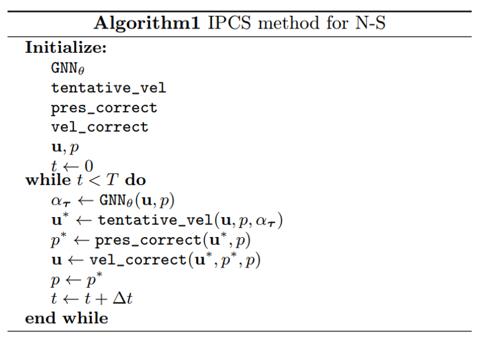
 In this algorithm, the GNN model is included to predict turbulence model parameters. And since the GNN model is written in the AD framework, no further work is required to enable gradient backpropagation. However, for the next three functions, tentative_vel, pres_correct, vel_correct, which are external routines and not known by the AD framework, a custom VJP for each of the PDE solution steps should be implemented.

  The PDE solver can be written generally as follows:
$x=$PDE_solve$(m),$
where x is state variables, such as pressure and velocity, and m is learnable model parameters.

Here we should implement a custom VJP:
$y_m=$PDE_solve_vjp$(y_x,m),$
where subscript represents partial differentiation.

The forward PDE-solving operations can be simplified into solving the linear system:
$A(m)x=b(m),$
where A and b represent the discretized left hand side (LHS) and right hand side (RHS) of the PDE respectively.

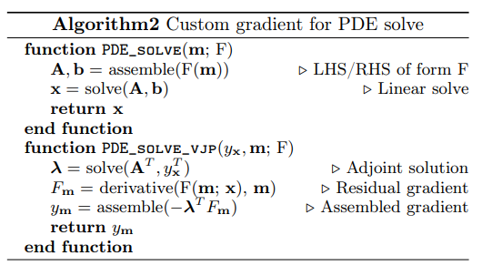
With this description, we can implement PDE_solve_vjp using the discrete adjoint method. Using the discrete adjoint method, the total derivative of y can be calculated as follows:
$\frac{dy}{dm}=-\lambda^T(A_mx-b_m),$
where $\lambda$ is the solution to the adjoint equation given by $A^T\lambda=y_x^T.$

The overall procedure for solving PDE and calculating custom VJP is shown below: